Robust and clustered standard errors with R
As you read in chapter 13.3 of The Effect, your standard errors in regressions are probably wrong. And as you read in the article by Guido Imbens, we want accurate standard errors because we should be focusing on confidence intervals when reporting our findings because nobody actually cares about or understands p-values.
So why are our standard errors wrong, and how do we fix them?
First, let’s make a model that predicts penguin weight based on bill length, flipper length, and species. We’ll use our regular old trusty lm() for an OLS model with regular standard errors.
library(tidyverse)       # For ggplot, dplyr, and friends
library(broom)           # Convert model objects into data frames
library(palmerpenguins)  # Our favorite penguin data

# Get rid of rows with missing values
penguins <- penguins %>% drop_na(sex)
model1 <- lm(body_mass_g ~ bill_length_mm + flipper_length_mm + species,
             data = penguins)
tidy(model1, conf.int = TRUE)
## # A tibble: 5 × 7
##   term              estimate std.error statistic  p.value conf.low conf.high
##   <chr>                <dbl>     <dbl>     <dbl>    <dbl>    <dbl>     <dbl>
## 1 (Intercept)        -3864.     534.       -7.24 3.18e-12  -4914.    -2814.
## 2 bill_length_mm        60.1      7.21      8.34 2.06e-15     45.9      74.3
## 3 flipper_length_mm     27.5      3.21      8.58 3.77e-16     21.2      33.9
## 4 speciesChinstrap    -732.      82.1      -8.93 3.22e-17   -894.     -571.
## 5 speciesGentoo        113.      89.2       1.27 2.05e- 1    -62.2     289.
A 1 mm increase in bill length is associated with a 60.1 g increase in penguin weight, on average. This is significantly significant and different from zero (p < 0.001), and the confidence interval ranges between 45.9 and 74.3, which means that we’re 95% confident that this range captures the true population parameter (this is a frequentist interval since we didn’t do any Bayesian stuff, so we have to talk about the confidence interval like a net and use awkward language).
This confidence interval is the coefficient estimate ± (1.96 × the standard error) (or 60.1 ± (1.96 × 7.21)), so it’s entirely dependent on the accuracy of the standard error. One of the assumptions of this estimate and its corresponding standard error is that the residuals of the regression (i.e. the distance from the predicted values and the actual values—remember this plot from Session 2) must not have any patterns in them. The official name for this assumption is that the errors in an OLS must be homoskedastic (or exhibit homoskedasticity). If errors are heteroskedastic—if the errors aren’t independent from each other, if they aren’t normally distributed, and if there are visible patterns in them—your standard errors (and confidence intervals) will be wrong.
Checking for heteroskedasticity
How do you know if your errors are homoskedastic of heterosketastic though?
The easiest way for me (and most people probably) is to visualize the residuals and see if there are any patterns. First, we can use augment() to calculate the residuals for each observation in the original penguin data and then make a scatterplot that puts the actual weight on the x-axis and the residuals on the y-axis.
# Plug the original data into the model and find fitted values and
# residuals/errors
fitted_data <- augment(model1, data = penguins)
# Look at relationship between fitted values and residuals
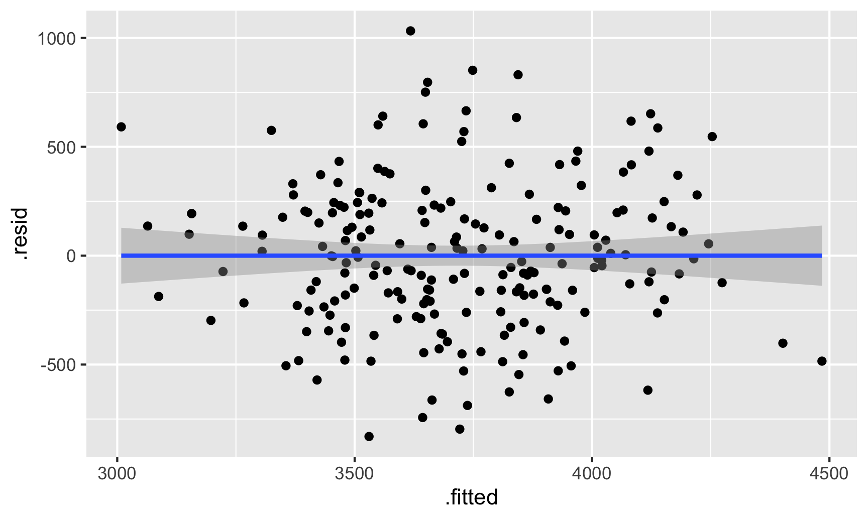
ggplot(fitted_data, aes(x = .fitted, y = .resid)) +
geom_point() +
geom_smooth(method = "lm")
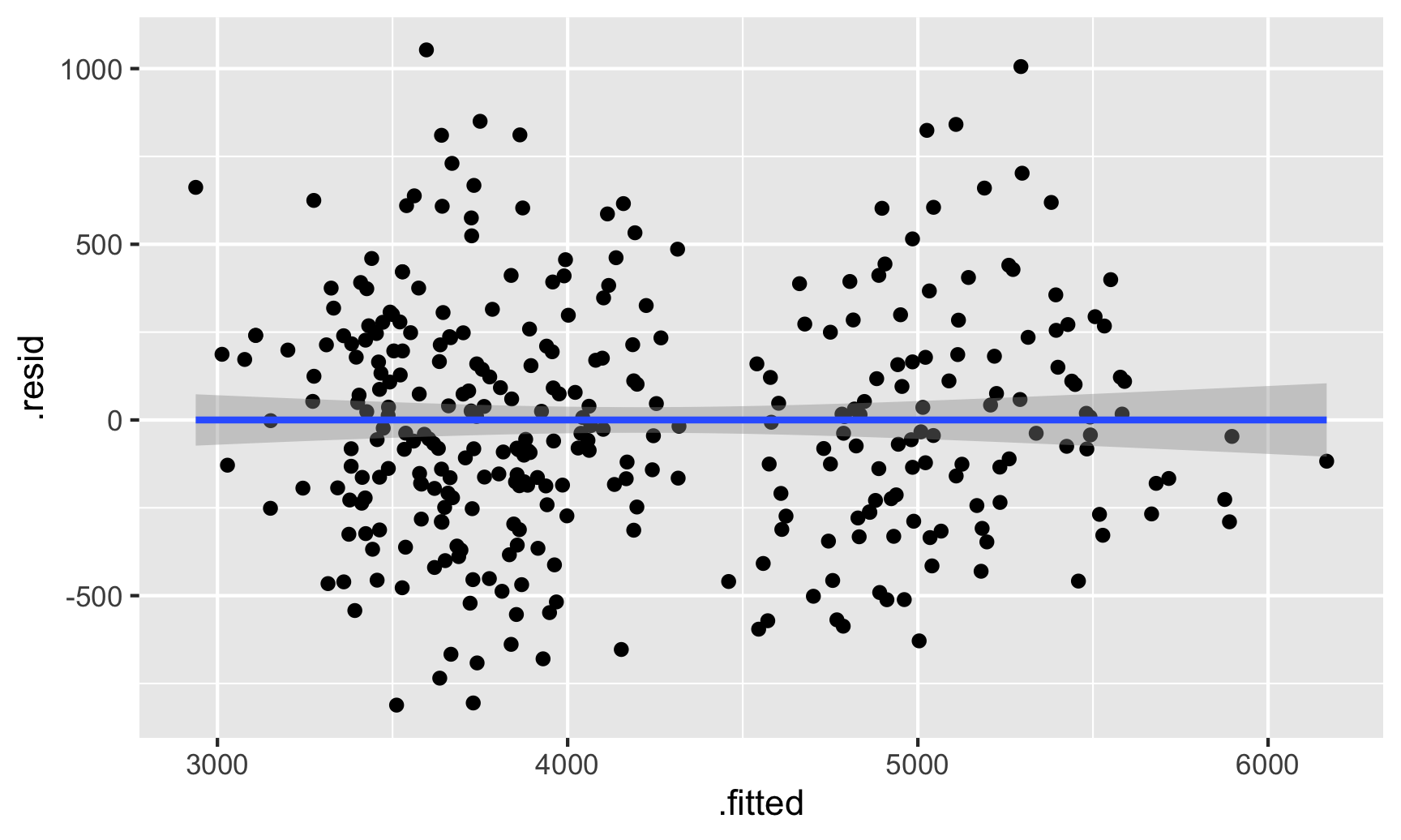
There seems to be two clusters of points here, which is potentially a sign that the errors aren’t independent of each other—there might be a systematic pattern in the errors. We can confirm this if we color the points by species:
ggplot(fitted_data, aes(x = .fitted, y = .resid)) +
  geom_point(aes(color = species)) +
  geom_smooth(method = "lm")
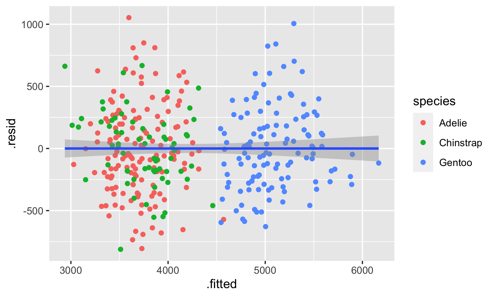
And there are indeed species-based clusters within the residuals! We can see this if we look at the distribution of the residuals too. For OLS assumptions to hold—and for our standard errors to be correct—this should be normally distributed:
ggplot(fitted_data, aes(x = .resid)) +
  geom_histogram(binwidth = 100, color = "white", boundary = 3000)
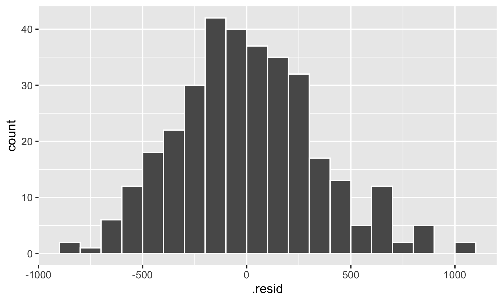
This looks fairly normal, though there are some more high residual observations (above 500) than we’d expect. That’s likely because the data isn’t actually heteroskedastic—it’s just clustered, and this clustering structure within the residuals means that our errors (and confidence intervals and p-values) are going to be wrong.
In this case the residual clustering creates a fairly obvious pattern. Just for fun, let’s ignore the Gentoos and see what residuals without clustering can look like. The residuals here actually look fairly random and pattern-free:
model_no_gentoo <- lm(body_mass_g ~ bill_length_mm + flipper_length_mm + species,
                      data = filter(penguins, species != "Gentoo"))

fitted_sans_gentoo <- augment(model_no_gentoo,
                              filter(penguins, species != "Gentoo"))

ggplot(fitted_sans_gentoo, aes(x = .fitted, y = .resid)) +
  geom_point() +
  geom_smooth(method = "lm")
We can do a neat little visual test for this. Let’s shuffle the residuals a bunch of times and make scatterplots with those shuffled values. If we can’t spot the actual residual plot among the shuffled ones, we can be fairly confident that there aren’t any patterns. The nullabor package makes this easy, allowing us to create a lineup of shuffled plots with the real residual plot mixed in there somewhere.
library(nullabor)

set.seed(1234)  # Shuffle these the same way every time

shuffled_residuals <- lineup(null_lm(body_mass_g ~ bill_length_mm + flipper_length_mm + species,
                                     method = "rotate"),
                             true = fitted_sans_gentoo,
                             n = 9)
## decrypt("h8RX 5IvI ne TAynvnAe kk")

ggplot(shuffled_residuals, aes(x = .fitted, y = .resid)) +
  geom_point() +
  facet_wrap(vars(.sample))
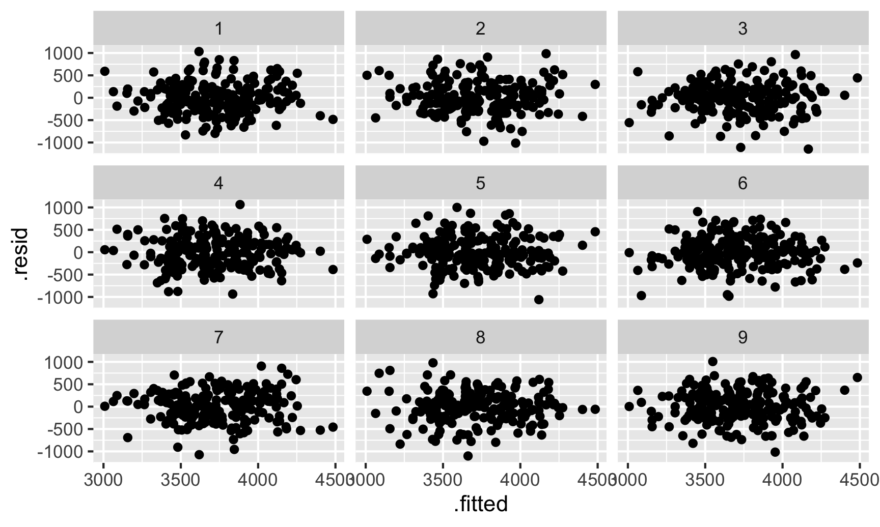
Which one is the actual residual plot? There’s no easy way to tell. That cryptic decrypt(...) thing is a special command that will tell us which plot is the correct one:
decrypt("sD0f gCdC En JP2EdEPn ZZ")
## Warning in decrypt("sD0f gCdC En JP2EdEPn ZZ"): NAs introduced by coercion
## [1] "OUxI EVkV ci CD3ckcDi  NA"
The fact that we can’t tell is a good sign that the residuals are homoskedastic and independent and that we don’t need to worry much about correcting the errors.
Adjusting standard errors
However, often you will see patterns or clusters in the residuals, which means you need to make some adjustments to the errors to ensure they’re accurate. In chapter 13.3 of The Effect you read about a bunch of different mathy ways to make these adjustments, and people get PhDs and write whole dissertations on new fancy ways to adjust standard errors. I’m not super interested in the deeper mathy mechanics of error adjustment, and most people aren’t either, so statistical software packages generally try to make it easy to make these adjustments without needing to think about the deeper math.
If you’re familiar with Stata, you can get robust standard errors like this:
# Run this in R first to export the penguins data as a CSV
write_csv("~/Desktop/penguins.csv")
/* Stata stuff */

import delimited "~/Desktop/penguins.csv", clear

encode species, generate(species_f)  /* Make species a factor /*

reg body_mass_g bill_length_mm flipper_length_mm i.species_f, robust

/*
Linear regression                               Number of obs     =        333
                                                F(4, 328)         =     431.96
                                                Prob > F          =     0.0000
                                                R-squared         =     0.8243
                                                Root MSE          =     339.57
-----------------------------------------------------------------------------------
                  |               Robust
      body_mass_g |      Coef.   Std. Err.      t    P>|t|     [95% Conf. Interval]
------------------+----------------------------------------------------------------
   bill_length_mm |   60.11733   6.429263     9.35   0.000     47.46953    72.76512
flipper_length_mm |   27.54429   3.054304     9.02   0.000     21.53579    33.55278
                  |
        species_f |
       Chinstrap  |  -732.4167     75.396    -9.71   0.000    -880.7374    -584.096
          Gentoo  |   113.2541   88.27028     1.28   0.200    -60.39317    286.9014
                  |
            _cons |  -3864.073   500.7276    -7.72   0.000    -4849.116   -2879.031
-----------------------------------------------------------------------------------
*/
And you can get clustered robust standard errors like this:
reg body_mass_g bill_length_mm flipper_length_mm i.species_f, cluster(species_f)

/*
Linear regression                               Number of obs     =        333
                                                F(1, 2)           =          .
                                                Prob > F          =          .
                                                R-squared         =     0.8243
                                                Root MSE          =     339.57
                                   (Std. Err. adjusted for 3 clusters in species_f)
-----------------------------------------------------------------------------------
                  |               Robust
      body_mass_g |      Coef.   Std. Err.      t    P>|t|     [95% Conf. Interval]
------------------+----------------------------------------------------------------
   bill_length_mm |   60.11733   12.75121     4.71   0.042     5.253298    114.9814
flipper_length_mm |   27.54429   4.691315     5.87   0.028     7.359188    47.72939
                  |
        species_f |
       Chinstrap  |  -732.4167   116.6653    -6.28   0.024    -1234.387   -230.4463
          Gentoo  |   113.2541   120.5977     0.94   0.447    -405.6361    632.1444
                  |
            _cons |  -3864.073   775.9628    -4.98   0.038    -7202.772   -525.3751
-----------------------------------------------------------------------------------
*/
Basically add , robust (or even just ,r) or cluster(whatever) to the end of the regression command.
Doing this in R is a little trickier since our favorite standard lm() command doesn’t have built-in support for robust or clustered standard errors, but there are some extra packages that make it really easy to do. Let’s look at three different ways.
sandwich and coeftest()
One way to adjust errors is to use the sandwich package, which actually handles the standard error correction behind the scenes for most of the other approaches we’ll look at. sandwich comes with a bunch of standard error correction functions, like vcovHC() for heteroskedasticity-consistent (HC) errors, vcovHAC() for heteroskedastiticy- and autocorrelation-consistent (HAC) errors, and vcovCL() for clustered errors (see their website for all the different ones). Within each of these different functions, there are different types (again, things that fancy smart statisticians figure out). If you want to replicate Stata’s , robust option exactly, you can use vcovHC(type = "HC1").
You can use these correction functions as an argument to the coeftest() function, the results of which conveniently work with tidy() and other broom functions. Here’s how we can get robust standard errors for our original penguin model (model1):
library(sandwich)  # Adjust standard errors
library(lmtest)    # Recalculate model errors with sandwich functions with coeftest()

# Robust standard errors with lm()
model1_robust <- coeftest(model1,
                          vcov = vcovHC)

# Stata's robust standard errors with lm()
model1_robust_stata <- coeftest(model1,
                                vcov = vcovHC,
                                type = "HC1")

tidy(model1_robust) %>% filter(term == "bill_length_mm")
## # A tibble: 1 × 5
##   term           estimate std.error statistic  p.value
##   <chr>             <dbl>     <dbl>     <dbl>    <dbl>
## 1 bill_length_mm     60.1      6.52      9.22 3.67e-18

tidy(model1_robust_stata) %>% filter(term == "bill_length_mm")
## # A tibble: 1 × 5
##   term           estimate std.error statistic  p.value
##   <chr>             <dbl>     <dbl>     <dbl>    <dbl>
## 1 bill_length_mm     60.1      6.43      9.35 1.40e-18
Those errors shrunk a little, likely because just using robust standard errors here isn’t enough. Remember that there are clear clusters in the residuals (Gentoo vs. not Gentoo), so we’ll actually want to cluster the errors by species. vcovCL() lets us do that:
# Clustered robust standard errors with lm()
model1_robust_clustered <- coeftest(model1,
                                    vcov = vcovCL,
                                    type = "HC1",
                                    cluster = ~species)

tidy(model1_robust_clustered, conf.int = TRUE) %>%
  filter(term == "bill_length_mm")
## # A tibble: 1 × 7
##   term           estimate std.error statistic    p.value conf.low conf.high
##   <chr>             <dbl>     <dbl>     <dbl>      <dbl>    <dbl>     <dbl>
## 1 bill_length_mm     60.1      12.8      4.71 0.00000359     35.0      85.2
Those errors are huge now, and the confidence interval ranges from 35 to 85! That’s because we’re now accounting for the clustered structure in the errors.
But we’re still not getting the same results as the clustered robust errors from Stata (or as feols() and lm_robust() below). This is because the data we’re working with here has a small number of clusters and coeftest()/vcovCL() doesn’t deal with that automatically (but Stata, feols(), and lm_robust() all do—see this section about it in the documentation for feols()). To fix this, we need to specify the number of degrees of freedom in the coeftest() function. There are three species/clusters in this data, so the degrees of freedom is 1 less than that, or 2.
# Clustered robust standard errors with lm(), correcting for small sample
model1_robust_clustered_corrected <- coeftest(model1,
                                              vcov = vcovCL,
                                              type = "HC1",
                                              df = 2,  # There are 3 species, so 3-1 = 2
                                              cluster = ~species)

tidy(model1_robust_clustered_corrected, conf.int = TRUE) %>%
  filter(term == "bill_length_mm")
## # A tibble: 1 × 7
##   term           estimate std.error statistic p.value conf.low conf.high
##   <chr>             <dbl>     <dbl>     <dbl>   <dbl>    <dbl>     <dbl>
## 1 bill_length_mm     60.1      12.8      4.71  0.0422     5.25      115.
There we go. Now we have absolutely massive confidence intervals ranging from 5 to 115. Who even knows what the true parameter is?! Our net probably caught it.
fixest and feols()
Standard error adjustment with the functions from sandwich and coeftest() works fine, but it requires multiple steps: (1) create a model with lm(), and (2) feed that model to coeftest(). It would be great if we could do that all at the same time in one command! Fortunately there are a few R packages that let us do this.
The feols() function from the fixest package was designed for OLS models that have lots of fixed effects (i.e. indicator variables), and it handles lots of fixed effects really really fast. It can also handle instrumental variables (which we’ll get to later in the semester). It’s a fantastic way to run models in R. It uses the same formula syntax as lm(), but with one extra feature: you can put fixed effects (again, indicator variables) after a | to specify that the variables are actually fixed effects. This (1) speeds up model estimation, and (2) hides the fixed effects from summary() and tidy() output, which is super convenient if you’re using something like county, state, or country fixed effects and you don’t want to see dozens or hundreds of extra rows in the regression output.
It includes an argument vcov for specifying how you want to handle the standard errors, and you can use lots of different options. Here we’ll make two models: one with heteroskedastic robust SEs (basically what Stata uses, or like vcovHC() in sandwich), and one with clustered robust standard errors (similar to vcovCL() in sandwich):
library(fixest)  # Run models with feols()

# Because species comes after |, it's being treated as a fixed effect
model_feols_hetero <- feols(body_mass_g ~ bill_length_mm + flipper_length_mm | species,
                            vcov = "hetero",
                            data = penguins)

tidy(model_feols_hetero) %>% filter(term == "bill_length_mm")
## # A tibble: 1 × 5
##   term           estimate std.error statistic  p.value
##   <chr>             <dbl>     <dbl>     <dbl>    <dbl>
## 1 bill_length_mm     60.1      6.43      9.35 1.40e-18

model_feols_clustered <- feols(body_mass_g ~ bill_length_mm + flipper_length_mm | species,
                               cluster = ~ species,
                               data = penguins)

tidy(model_feols_clustered, conf.int = TRUE) %>% filter(term == "bill_length_mm")
## # A tibble: 1 × 7
##   term           estimate std.error statistic p.value conf.low conf.high
##   <chr>             <dbl>     <dbl>     <dbl>   <dbl>    <dbl>     <dbl>
## 1 bill_length_mm     60.1      12.7      4.73  0.0419     5.42      115.
We get basically the same standard errors we did before with coeftest(lm(), vcov = ...), only now we did it all in one step.
estimatr and lm_robust()
The lm_robust() function in the estimatr package also allows you to calculate robust standard errors in one step using the se_type argument. See the documentation for all the possible options. Here we can replicate Stata’s standard errors by using se_type = "stata" (se_type = "HC1" would do the same thing). lm_robust() also lets you specify fixed effects separately so that they’re hidden in the results, but instead of including them in the formula like we did with feols(), we have to use the fixed_effects argument.
library(estimatr)  # Run models with lm_robust()

model_lmrobust_clustered <- lm_robust(body_mass_g ~ bill_length_mm + flipper_length_mm,
                                      fixed_effects = ~ species,
                                      se_type = "stata",
                                      clusters = species,
                                      data = penguins)

tidy(model_lmrobust_clustered, conf.int = TRUE) %>% filter(term == "bill_length_mm")
##             term estimate std.error statistic p.value conf.low conf.high df     outcome
## 1 bill_length_mm       60        13       4.7   0.042      5.3       115  2 body_mass_g
On-the-fly SE adjustment
While it’s neat that we can specify standard errors directly in feols() and lm_robust(), it’s sometimes (almost always) a good idea to actually not adjust SEs within the models themselves and instead make the adjustments after you’ve already fit the model. This is especially the case if you have a more complex model that takes a while to run. Note how we ran a couple different feols() models previously—it would be nice if we could just run the model once and then choose whatever standard error adjustments we want later. This is what we already did with coeftest(model, vcov = ...). We can do similar things with feols(). Watch how we can specify the standard error options and clusters inside tidy() directly, with just one model!
model_feols_basic <- feols(body_mass_g ~ bill_length_mm + flipper_length_mm | species,
                           data = penguins)

tidy(model_feols_basic, se = "hetero") %>% filter(term == "bill_length_mm")
## # A tibble: 1 × 5
##   term           estimate std.error statistic  p.value
##   <chr>             <dbl>     <dbl>     <dbl>    <dbl>
## 1 bill_length_mm     60.1      6.43      9.35 1.40e-18

tidy(model_feols_basic, cluster = "species") %>% filter(term == "bill_length_mm")
## # A tibble: 1 × 5
##   term           estimate std.error statistic p.value
##   <chr>             <dbl>     <dbl>     <dbl>   <dbl>
## 1 bill_length_mm     60.1      12.7      4.73  0.0419
The modelsummary() function from the modelsummary package also lets us make SE adjustments on the fly. Check this out—with just one basic model with lm(), we can get all these different kinds of standard errors!
library(modelsummary)  # Make nice tables and plots for models

model_basic <- lm(body_mass_g ~ bill_length_mm + flipper_length_mm + species,
                  data = penguins)

# Add an extra row with the error names
se_info <- tibble(term = "Standard errors", "Regular", "Robust", "Stata", "Clustered by species")

modelsummary(model_basic,
             # Specify how to robustify/cluster the model
             vcov = list("iid", "robust", "stata", function(x) vcovCL(x, cluster = ~ species)),
             # Get rid of other coefficients and goodness-of-fit (gof) stats
             coef_omit = "species|flipper|Intercept", gof_omit = ".*",
             add_rows = se_info)
| Model 1 | Model 2 | Model 3 | Model 4 | |
|---|---|---|---|---|
| bill_length_mm | 60.117 | 60.117 | 60.117 | 60.117 |
| (7.207) | (6.519) | (6.429) | (12.751) | |
| Standard errors | Regular | Robust | Stata | Clustered by species |
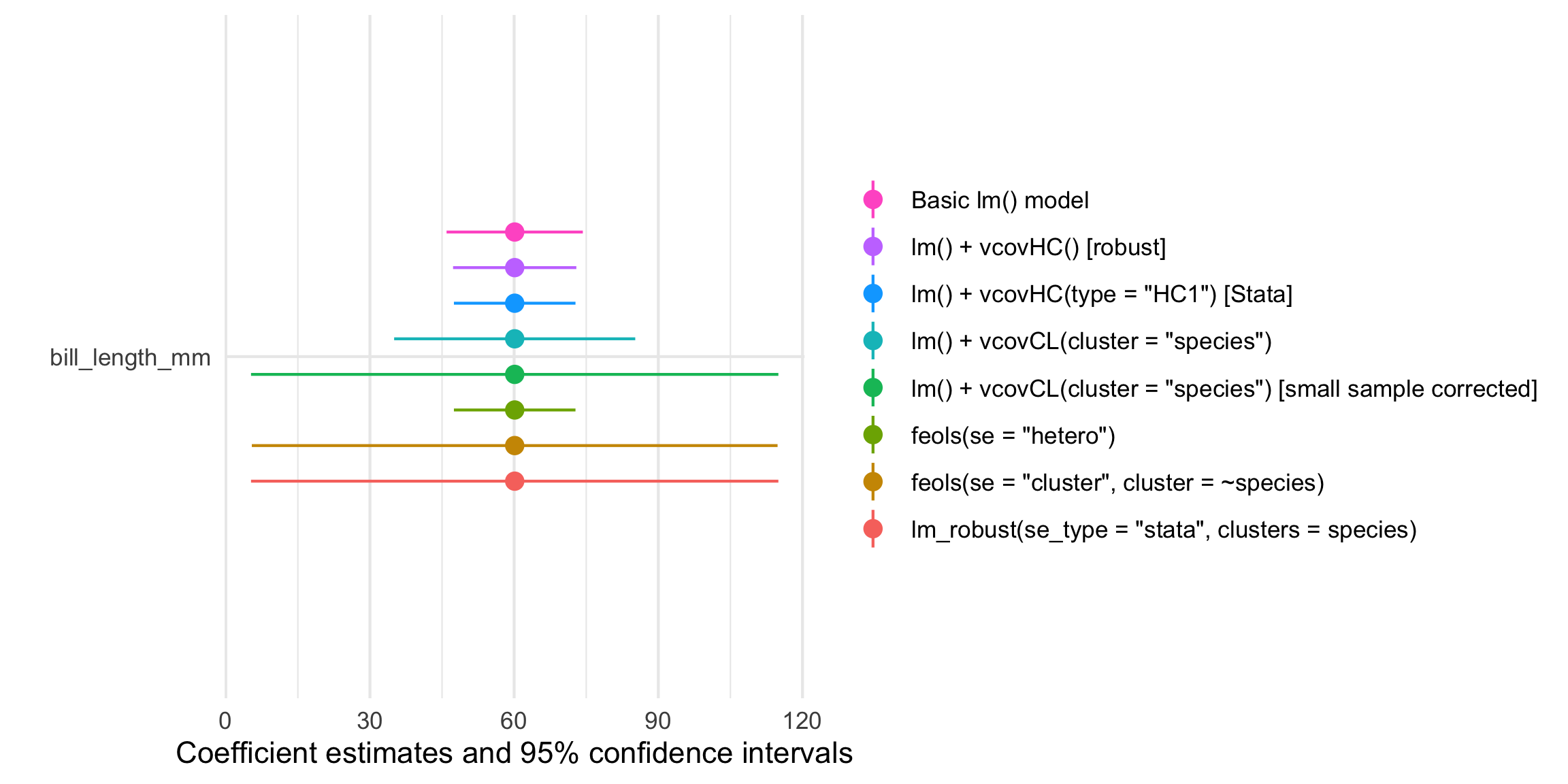
Plot all these confidence intervals
The modelsummary package also comes with a modelplot() function that will create a coefficient plot showing the point estimates and 95% confidence intervals. Look at all these different standard errors!
modelplot(
  list('lm_robust(se_type = "stata", clusters = species)' = model_lmrobust_clustered,
       'feols(se = "cluster", cluster = ~species)' = model_feols_clustered,
       'feols(se = "hetero")' = model_feols_hetero,
       'lm() + vcovCL(cluster = "species") [small sample corrected]' = model1_robust_clustered_corrected,
       'lm() + vcovCL(cluster = "species")' = model1_robust_clustered,
       'lm() + vcovHC(type = "HC1") [Stata]' = model1_robust_stata,
       "lm() + vcovHC() [robust]" = model1_robust,
       "Basic lm() model" = model1),
  coef_omit = "species|flipper|Intercept") +
  guides(color = guide_legend(reverse = TRUE))