Welcome to R, RStudio, and the tidyverse!
Part 1: The basics of R and dplyr
For this week’s problem set, you need to work through a few of RStudio’s introductory primers. You’ll do these in your browser and type code and see results there.
You’ll learn some of the basics of R, as well as some powerful methods for manipulating data with the dplyr package.
Complete these primers. It seems like there are a lot, but they’re short and go fairly quickly (especially as you get the hang of the syntax). Also, I have no way of seeing what you do or what you get wrong or right, and that’s totally fine! If you get stuck and want to skip some (or if it gets too easy), go right ahead and skip them!
- The Basics
- Work with Data
- Visualize Data
- Tidy Your Data
gather() is now pivot_longer() and spread() is now pivot_wider(). The syntax for these pivot_*() functions is slightly different from what it was in gather() and spread(), so you can’t just replace the names. Fortunately, both gather() and spread() still work and won’t go away for a while, so you can still use them as you learn about reshaping and tidying data. It would be worth learning how the newer pivot_*() functions work, eventually, though (see here for examples).
The content from these primers comes from the (free and online!) book R for Data Science by Garrett Grolemund and Hadley Wickham. I highly recommend the book as a reference and for continuing to learn and use R in the future.
Part 2: Getting familiar with RStudio
The RStudio primers you just worked through are a great introduction to writing and running R code, but you typically won’t type code in a browser when you work with R. Instead, you’ll use a nicer programming environment like RStudio, which lets you type and save code in scripts, run code from those scripts, and see the output of that code, all in the same program.
To get familiar with RStudio, watch this video (it’s from PMAP 8921, but the content still applies here):
Part 3: RStudio Projects
One of the most powerful and useful aspects of RStudio is its ability to manage projects.
When you first open R, it is “pointed” at some folder on your computer, and anything you do will be relative to that folder. The technical term for this is a “working directory.”
When you first open RStudio, look in the area right at the top of the Console pane to see your current working directory. Most likely you’ll see something cryptic: ~/
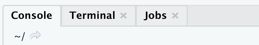
That tilde sign (~) is a shortcut that stands for your user directory. On Windows this is C:\Users\your_user_name\; on macOS this is /Users/your_user_name/. With the working directory set to ~/, R is “pointed” at that folder, and anything you save will end up in that folder, and R will expect any data that you load to be there too.
It’s always best to point R at some other directory. If you don’t use RStudio, you need to manually set the working directory to where you want it with setwd(), and many R scripts in the wild include something like setwd("C:\\Users\\bill\\Desktop\\Important research project") at the beginning to change the directory. THIS IS BAD THOUGH (see here for an explanation). If you ever move that directory somewhere else, or run the script on a different computer, or share the project with someone, the path will be wrong and nothing will run and you will be sad.
The best way to deal with working directories with RStudio is to use RStudio Projects. These are special files that RStudio creates for you that end in a .Rproj extension. When you open one of these special files, a new RStudio instance will open up and be pointed at the correct directory automatically. If you move the folder later or open it on a different computer, it will work just fine and you will not be sad.
Read this super short chapter on RStudio projects to learn how to create and use them
In general, you can create a new project by going to File > New Project > New Directory > Empty Project, which will create a new folder on your computer that is empty except for a single .Rproj file. Double click on that file to open an RStudio instance that is pointed at the correct folder.
Part 4: Getting familiar with R Markdown
To ensure that the analysis and graphics you make are reproducible, you’ll do the majority of your work in this class using R Markdown files.
Do the following things:
- Watch this video:
-
Skim through the content at these pages:
- Using Markdown
- Using R Markdown
- How it Works
- Code Chunks
- Inline Code
- Markdown Basics (The R Markdown Reference Guide is super useful here.)
- Output Formats
-
Watch this video (again, it’s from PMAP 8921, but the content works for this class):